Hypothesis Testing

Using computer simulation. Based on examples from the infer package. Code for Quiz 13.

Load the R packages we will use:

library(tidyverse)
library(infer)
library(skimr)

Question: t-test

• The data this quiz uses is a subset of HR

  • Look at the variable definitions

• Note that the variables evaluation and salary have been recoded to be represented as words instead of numbers

  • Set random seed generator to 123

set.seed(123)

hr_2_tidy.csv is the name of your data subset

-Read it into and assign to hr

• Note: col_types = “fddfff” defines the column types factor-double-double-factor-factor-factor

hr  <- read_csv("https://estanny.com/static/week13/data/hr_3_tidy.csv", 
                col_types = "fddfff")

use skim to summarize the data in hr

skim(hr)

Table 1: Data summary

Name	hr
Number of rows	500
Number of columns	6
_______________________
Column type frequency:
factor	4
numeric	2
________________________
Group variables	None

Variable type: factor

skim_variable	n_missing	complete_rate	ordered	n_unique	top_counts
gender	0	1	FALSE	2	fem: 253, mal: 247
evaluation	0	1	FALSE	4	bad: 148, fai: 138, goo: 122, ver: 92
salary	0	1	FALSE	6	lev: 98, lev: 87, lev: 87, lev: 86
status	0	1	FALSE	3	fir: 196, pro: 172, ok: 132

Variable type: numeric

skim_variable	n_missing	complete_rate	mean	sd	p0	p25	p50	p75	p100	hist
age	0	1	39.41	11.33	20	29.9	39.35	49.1	59.9	▇▇▇▇▆
hours	0	1	49.68	13.24	35	38.2	45.50	58.8	79.9	▇▃▃▂▂

specify that hours is the variable of interest

hr %>% 
  specify(response = hours)

Response: hours (numeric)
# A tibble: 500 × 1
   hours
   <dbl>
 1  49.6
 2  39.2
 3  63.2
 4  42.2
 5  54.7
 6  54.3
 7  37.3
 8  45.6
 9  35.1
10  53  
# … with 490 more rows

hypothesize that the average hours worked is 48

hr  %>% 
  specify(response = hours)  %>% 
  hypothesize(null = "point", mu = 48)

Response: hours (numeric)
Null Hypothesis: point
# A tibble: 500 × 1
   hours
   <dbl>
 1  49.6
 2  39.2
 3  63.2
 4  42.2
 5  54.7
 6  54.3
 7  37.3
 8  45.6
 9  35.1
10  53  
# … with 490 more rows

generate 1000 replicates representing the null hypothesis

hr %>% 
  specify(response = hours)  %>% 
  hypothesize(null = "point", mu = 48)  %>% 
  generate(reps = 1000, type = "bootstrap")

Response: hours (numeric)
Null Hypothesis: point
# A tibble: 500,000 × 2
# Groups:   replicate [1,000]
   replicate hours
       <int> <dbl>
 1         1  34.5
 2         1  33.6
 3         1  35.6
 4         1  78.2
 5         1  52.7
 6         1  77.0
 7         1  37.1
 8         1  41.9
 9         1  62.7
10         1  38.8
# … with 499,990 more rows

calculate the distribution of statistics from the generated data - Assign the output null_t_distribution - Display null_t_distribution

null_t_distribution  <- hr  %>% 
  specify(response = age)  %>% 
  hypothesize(null = "point", mu = 48)  %>% 
  generate(reps = 1000, type = "bootstrap")  %>% 
  calculate(stat = "t")
null_t_distribution

Response: age (numeric)
Null Hypothesis: point
# A tibble: 1,000 × 2
   replicate    stat
       <int>   <dbl>
 1         1  0.929 
 2         2  0.480 
 3         3 -0.0136
 4         4  0.435 
 5         5 -0.810 
 6         6 -1.06  
 7         7 -0.0470
 8         8  0.809 
 9         9  0.986 
10        10  0.199 
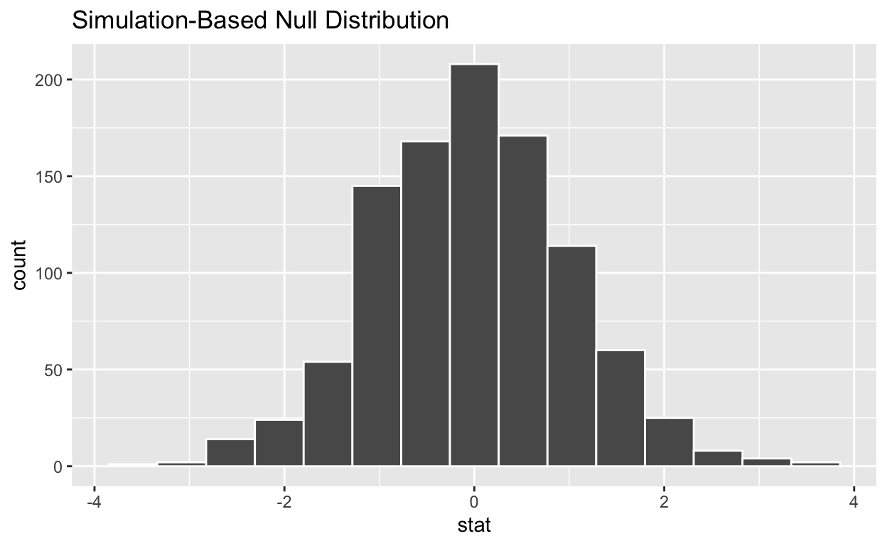
# … with 990 more rows

visualize the simulated null distribution

visualize(null_t_distribution)

calculate the statistic from your observed data

• Assign the output observed_t_statistic
• Display observed_t_statistic

observed_t_statistic  <- hr  %>%
  specify(response = hours)  %>% 
  hypothesize(null = "point", mu = 48)  %>%
  calculate(stat = "t")
observed_t_statistic

Response: hours (numeric)
Null Hypothesis: point
# A tibble: 1 × 1
   stat
  <dbl>
1  2.83

get_p_value from the simulated null distribution and the observed statistic

null_t_distribution  %>% 
  get_p_value(obs_stat = observed_t_statistic, direction = "two-sided")

# A tibble: 1 × 1
  p_value
    <dbl>
1   0.012

shade_p_value on the simulated null distribution

null_t_distribution  %>% 
  visualize() +
  shade_p_value(obs_stat = observed_t_statistic, direction = "two-sided")

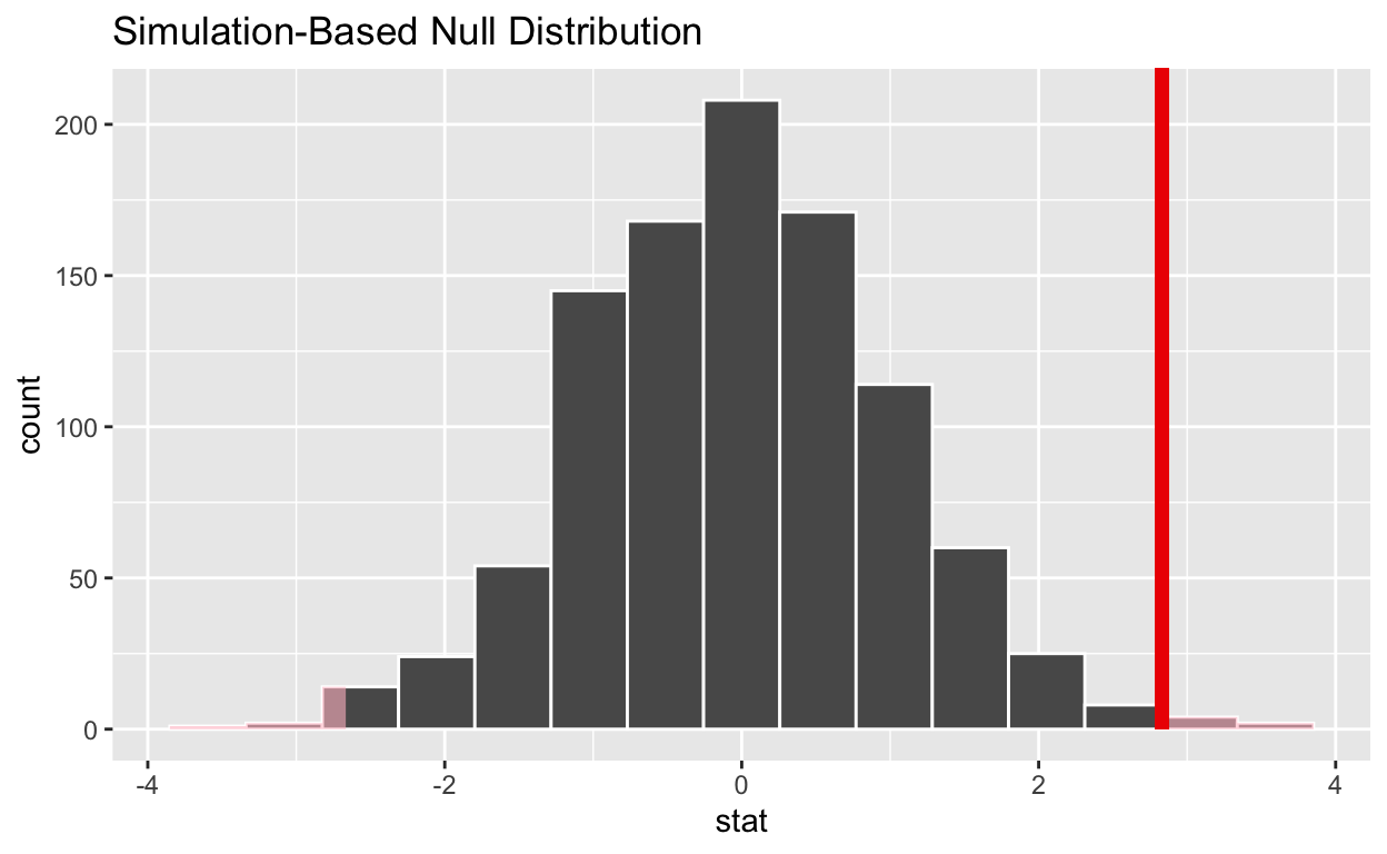
Is the p-value < 0.05? yes

Does your analysis support the null hypothesis that the true mean number of hours worked was 48? no

#Question 2: sample t-test

• Make sure you have installed and loaded the tidyverse, infer, and skimr packages Fill in the blanks:
• Put the command you use in the Rchunks in your Rmd file for this quiz.
• The data this quiz is a subset of HR
• Look at the variable definitions *Note that the variables evaluation and salary have been recoded to be represented as words instead of numbers hr_1_tidy.csv is the name of your data subset
• Read it into and assign to hr_2 *Note: col_types = “fddfff” defines the column types factor-double-double-factor-factor-factor

hr_1_tidy.csv is the name of your data subset

hr_2 <- read_csv("https://estanny.com/static/week13/data/hr_1_tidy.csv", 
                col_types = "fddfff")

#Q: Is the average number of hours worked the same for both genders in hr_2? - use skim to summarize the data in hr_2 by gender

hr_2 %>% 
  group_by(gender)  %>% 
  skim()

Table 2: Data summary

Name	Piped data
Number of rows	500
Number of columns	6
_______________________
Column type frequency:
factor	3
numeric	2
________________________
Group variables	gender

Variable type: factor

skim_variable	gender	n_missing	complete_rate	ordered	n_unique	top_counts
evaluation	female	0	1	FALSE	4	fai: 81, bad: 71, ver: 57, goo: 51
evaluation	male	0	1	FALSE	4	bad: 82, fai: 61, goo: 55, ver: 42
salary	female	0	1	FALSE	6	lev: 54, lev: 50, lev: 44, lev: 41
salary	male	0	1	FALSE	6	lev: 52, lev: 47, lev: 46, lev: 39
status	female	0	1	FALSE	3	fir: 96, pro: 87, ok: 77
status	male	0	1	FALSE	3	fir: 89, ok: 76, pro: 75

Variable type: numeric

skim_variable	gender	n_missing	complete_rate	mean	sd	p0	p25	p50	p75	p100	hist
age	female	0	1	41.78	11.50	20.5	32.15	42.35	51.62	59.9	▆▅▇▆▇
age	male	0	1	39.32	11.55	20.2	28.70	38.55	49.52	59.7	▇▇▆▇▆
hours	female	0	1	50.32	13.23	35.0	38.38	47.80	60.40	79.7	▇▃▃▂▂
hours	male	0	1	48.24	12.95	35.0	37.00	42.40	57.00	78.1	▇▂▂▁▂

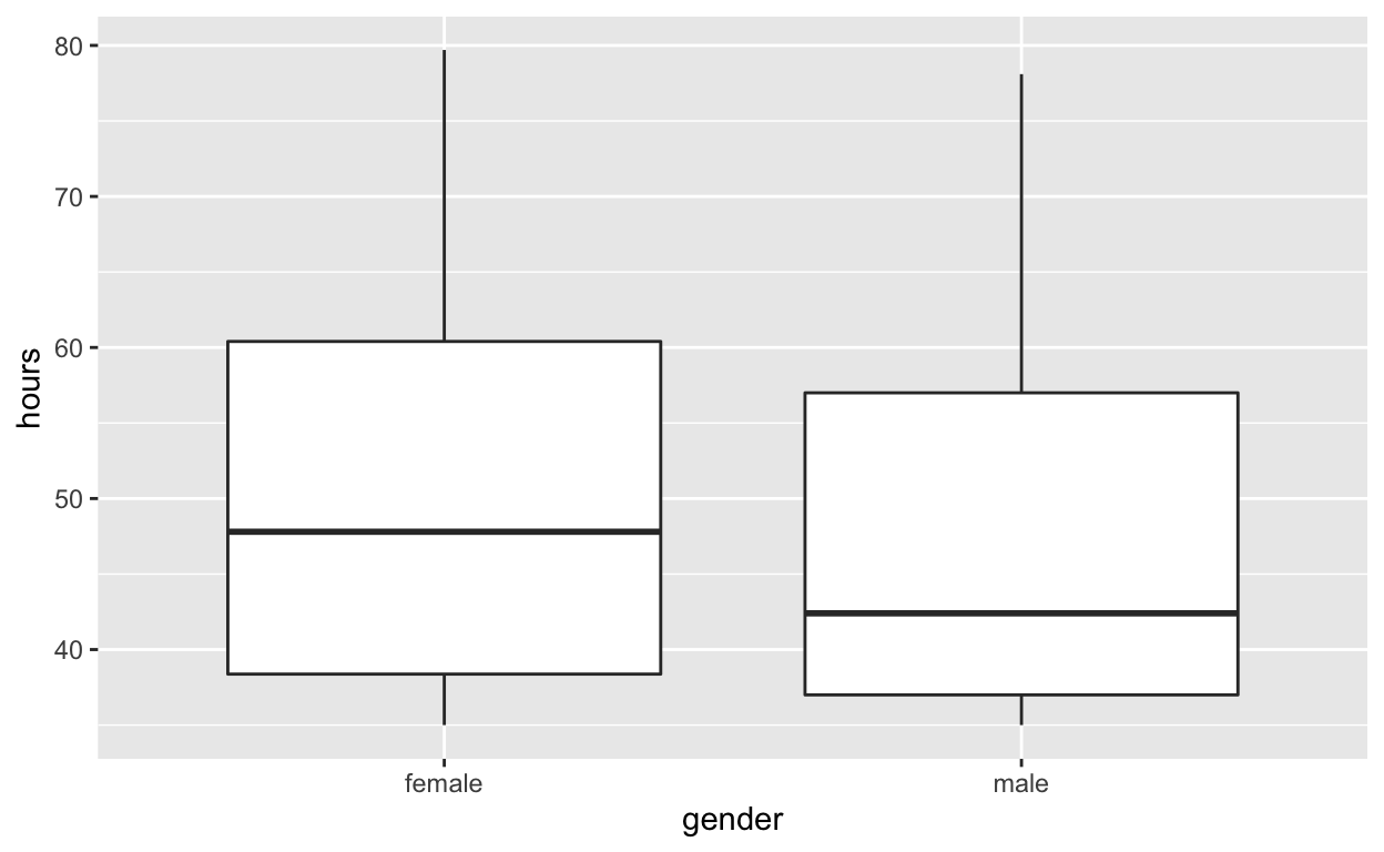
Use geom_boxplot to plot distributions of hours worked by gender

hr_2 %>% 
  ggplot(aes(x = gender, y = hours)) + 
  geom_boxplot()

specify the variables of interest are hours and gender

hr_2 %>% 
  specify(response = hours, explanatory = gender)

Response: hours (numeric)
Explanatory: gender (factor)
# A tibble: 500 × 2
   hours gender
   <dbl> <fct> 
 1  36.5 female
 2  55.8 female
 3  35   male  
 4  52   female
 5  35.1 male  
 6  36.3 female
 7  40.1 female
 8  42.7 female
 9  66.6 male  
10  35.5 male  
# … with 490 more rows

hypothesize that the number of hours worked and gender are independent

hr_2  %>% 
  specify(response = hours, explanatory = gender)  %>% 
  hypothesize(null = "independence")

Response: hours (numeric)
Explanatory: gender (factor)
Null Hypothesis: independence
# A tibble: 500 × 2
   hours gender
   <dbl> <fct> 
 1  36.5 female
 2  55.8 female
 3  35   male  
 4  52   female
 5  35.1 male  
 6  36.3 female
 7  40.1 female
 8  42.7 female
 9  66.6 male  
10  35.5 male  
# … with 490 more rows

generate 1000 replicates representing the null hypothesis

hr_2 %>% 
  specify(response = hours, explanatory = gender)  %>% 
  hypothesize(null = "independence")  %>% 
  generate(reps = 1000, type = "permute")

Response: hours (numeric)
Explanatory: gender (factor)
Null Hypothesis: independence
# A tibble: 500,000 × 3
# Groups:   replicate [1,000]
   hours gender replicate
   <dbl> <fct>      <int>
 1  36.4 female         1
 2  35.8 female         1
 3  35.6 male           1
 4  39.6 female         1
 5  35.8 male           1
 6  55.8 female         1
 7  63.8 female         1
 8  40.3 female         1
 9  56.5 male           1
10  50.1 male           1
# … with 499,990 more rows

calculate the distribution of statistics from the generated data

• Assign the output null_distribution_2_sample_permute
• Display null_distribution_2_sample_permute

null_distribution_2_sample_permute  <- hr_2 %>% 
  specify(response = hours, explanatory = gender)  %>% 
  hypothesize(null = "independence")  %>% 
  generate(reps = 1000, type = "permute")  %>% 
  calculate(stat = "t", order = c("female", "male"))

null_distribution_2_sample_permute

Response: hours (numeric)
Explanatory: gender (factor)
Null Hypothesis: independence
# A tibble: 1,000 × 2
   replicate   stat
       <int>  <dbl>
 1         1 -0.208
 2         2 -0.328
 3         3 -2.28 
 4         4  0.528
 5         5  1.60 
 6         6  0.795
 7         7  1.24 
 8         8 -3.31 
 9         9  0.517
10        10  0.949
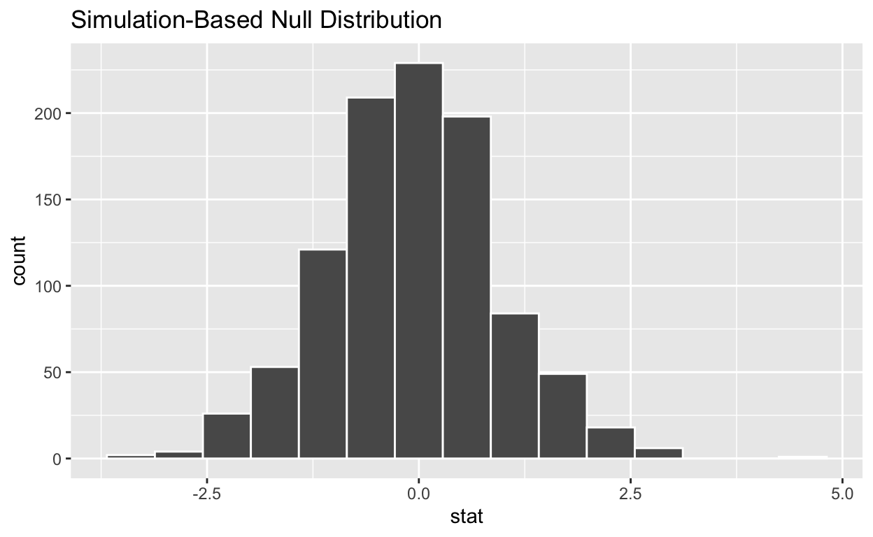
# … with 990 more rows

visualize the simulated null distribution

visualize(null_distribution_2_sample_permute)

calculate the statistic from your observed data

• Assign the output observed_t_2_sample_stat
• Display observed_t_2_sample_stat

observed_t_2_sample_stat  <- hr_2 %>%
  specify(response = hours, explanatory = gender)  %>% 
  calculate(stat = "t", order = c("female", "male"))

observed_t_2_sample_stat

Response: hours (numeric)
Explanatory: gender (factor)
# A tibble: 1 × 1
   stat
  <dbl>
1  1.78

get_p_value from the simulated null distribution and the observed statistic

null_t_distribution  %>% 
  get_p_value(obs_stat = observed_t_2_sample_stat, direction = "two-sided")

# A tibble: 1 × 1
  p_value
    <dbl>
1    0.08

shade_p_value on the simulated null distribution

null_t_distribution  %>% 
  visualize() +
  shade_p_value(obs_stat = observed_t_2_sample_stat, direction = "two-sided")

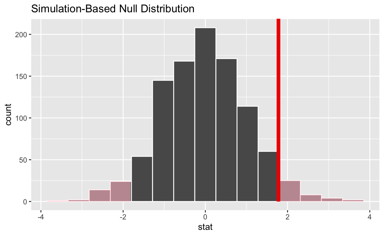
Is the p-value < 0.05? no

Does your analysis support the null hypothesis that the true mean number of hours worked by female and male employees was the same? yes

hr_2_tidy.csv is the name of your data subset

• Read it into and assign to hr_anova *Note: col_types = “fddfff” defines the column types factor-double-double-factor-factor-factor

hr_anova <- read_csv("https://estanny.com/static/week13/data/hr_2_tidy.csv", 
                col_types = "fddfff")

Q: Is the average number of hours worked the same for all three status (fired, ok and promoted) ?

use skim to summarize the data in hr_anova by status

hr_anova %>% 
  group_by(status)  %>% 
  skim()

Table 3: Data summary

Name	Piped data
Number of rows	500
Number of columns	6
_______________________
Column type frequency:
factor	3
numeric	2
________________________
Group variables	status

Variable type: factor

skim_variable	status	n_missing	complete_rate	ordered	n_unique	top_counts
gender	promoted	0	1	FALSE	2	mal: 90, fem: 89
gender	fired	0	1	FALSE	2	fem: 101, mal: 93
gender	ok	0	1	FALSE	2	mal: 73, fem: 54
evaluation	promoted	0	1	FALSE	4	goo: 70, ver: 62, fai: 24, bad: 23
evaluation	fired	0	1	FALSE	4	bad: 78, fai: 72, goo: 25, ver: 19
evaluation	ok	0	1	FALSE	4	bad: 53, fai: 46, ver: 15, goo: 13
salary	promoted	0	1	FALSE	6	lev: 42, lev: 42, lev: 39, lev: 34
salary	fired	0	1	FALSE	6	lev: 54, lev: 44, lev: 34, lev: 24
salary	ok	0	1	FALSE	6	lev: 32, lev: 31, lev: 26, lev: 19

Variable type: numeric

skim_variable	status	n_missing	complete_rate	mean	sd	p0	p25	p50	p75	p100	hist
age	promoted	0	1	40.63	11.25	20.4	30.75	41.10	50.25	59.9	▆▇▇▇▇
age	fired	0	1	40.03	11.53	20.3	29.45	40.40	50.08	59.9	▇▅▇▆▆
age	ok	0	1	38.50	11.98	20.3	28.15	38.70	49.45	59.9	▇▆▅▅▆
hours	promoted	0	1	59.21	12.66	35.0	49.75	58.90	70.65	79.9	▅▆▇▇▇
hours	fired	0	1	41.67	8.37	35.0	36.10	38.45	43.40	77.7	▇▂▁▁▁
hours	ok	0	1	47.35	10.86	35.0	37.10	45.70	54.50	78.9	▇▅▃▂▁

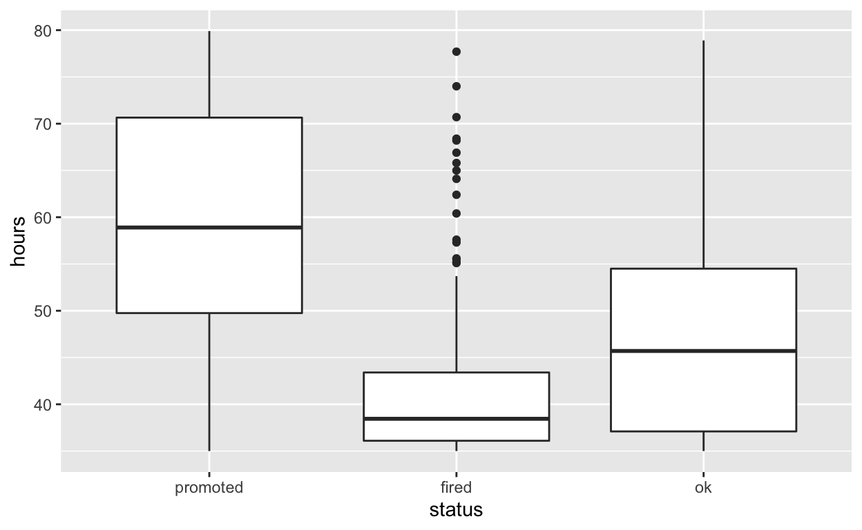
• Employees that were fired worked an average of 41.7 hours per week
• Employees that were okay worked an average of 48.0 hours per week
• Employees that were promoted worked an average of 59.3 hours per week

Use geom_boxplot to plot distributions of hours worked by status

hr_anova %>% 
  ggplot(aes(x = status, y = hours)) + 
  geom_boxplot()

specify the variables of interest are hours and status

hr_anova %>% 
  specify(response = hours, explanatory = status)

Response: hours (numeric)
Explanatory: status (factor)
# A tibble: 500 × 2
   hours status  
   <dbl> <fct>   
 1  78.1 promoted
 2  35.1 fired   
 3  36.9 fired   
 4  38.5 fired   
 5  36.1 fired   
 6  78.1 promoted
 7  76   promoted
 8  35.6 fired   
 9  35.6 ok      
10  56.8 promoted
# … with 490 more rows

hypothesize that the number of hours worked and status are independent

hr_anova  %>% 
  specify(response = hours, explanatory = status)  %>% 
  hypothesize(null = "independence")

Response: hours (numeric)
Explanatory: status (factor)
Null Hypothesis: independence
# A tibble: 500 × 2
   hours status  
   <dbl> <fct>   
 1  78.1 promoted
 2  35.1 fired   
 3  36.9 fired   
 4  38.5 fired   
 5  36.1 fired   
 6  78.1 promoted
 7  76   promoted
 8  35.6 fired   
 9  35.6 ok      
10  56.8 promoted
# … with 490 more rows

generate 1000 replicates representing the null hypothesis

hr_anova %>% 
  specify(response = hours, explanatory = status)  %>% 
  hypothesize(null = "independence")  %>% 
  generate(reps = 1000, type = "permute") 

Response: hours (numeric)
Explanatory: status (factor)
Null Hypothesis: independence
# A tibble: 500,000 × 3
# Groups:   replicate [1,000]
   hours status   replicate
   <dbl> <fct>        <int>
 1  41.9 promoted         1
 2  36.7 fired            1
 3  35   fired            1
 4  58.9 fired            1
 5  36.1 fired            1
 6  39.4 promoted         1
 7  54.3 promoted         1
 8  59.2 fired            1
 9  40.2 ok               1
10  35.3 promoted         1
# … with 499,990 more rows

calculate the distribution of statistics from the generated data

• Assign the output null_distribution_anova
• Display null_distribution_anova

null_distribution_anova <- hr_anova %>% 
  specify(response = hours, explanatory = status) %>% 
  hypothesize(null = ("independence")) %>% 
  generate(reps = 1000, type = "permute") %>% 
  calculate(stat = "F")
null_distribution_anova

Response: hours (numeric)
Explanatory: status (factor)
Null Hypothesis: independence
# A tibble: 1,000 × 2
   replicate  stat
       <int> <dbl>
 1         1 0.312
 2         2 2.85 
 3         3 0.369
 4         4 0.142
 5         5 0.511
 6         6 2.73 
 7         7 1.06 
 8         8 0.171
 9         9 0.310
10        10 1.11 
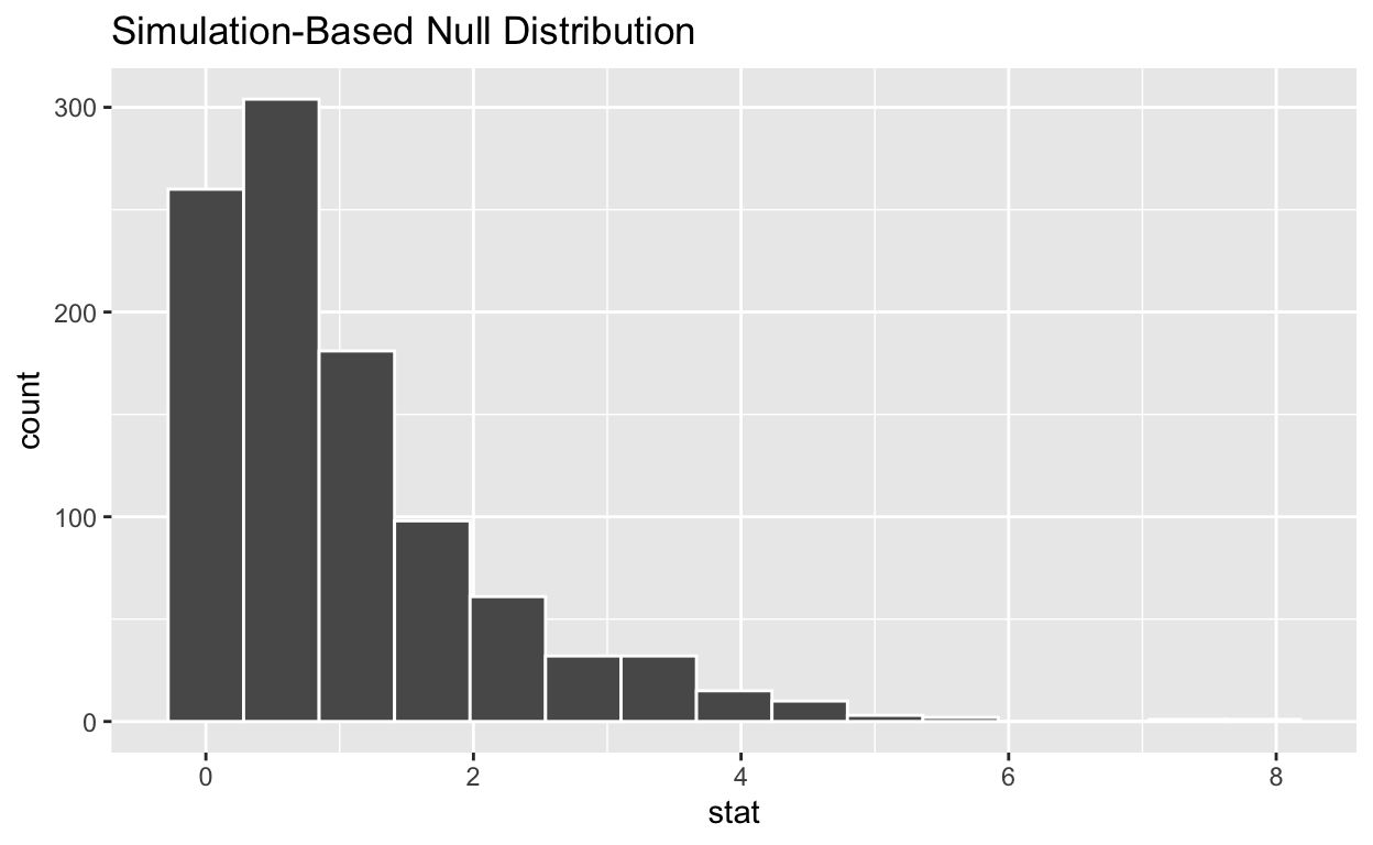
# … with 990 more rows

visualize the simulated null distribution

visualize(null_distribution_anova)

calculate the statistic from your observed data

• Assign the output observed_f_sample_stat
• Display observed_f_sample_stat

observed_f_sample_stat  <- hr_anova %>%
  specify(response = hours, explanatory = status)  %>% 
  calculate(stat = "F")

observed_f_sample_stat

Response: hours (numeric)
Explanatory: status (factor)
# A tibble: 1 × 1
   stat
  <dbl>
1  128.

get_p_value from the simulated null distribution and the observed statistic

null_distribution_anova  %>% 
  get_p_value(obs_stat = observed_f_sample_stat, direction = "greater")

# A tibble: 1 × 1
  p_value
    <dbl>
1       0

shade_p_value on the simulated null distribution

null_t_distribution  %>% 
  visualize() +
  shade_p_value(obs_stat = observed_f_sample_stat, direction = "greater")

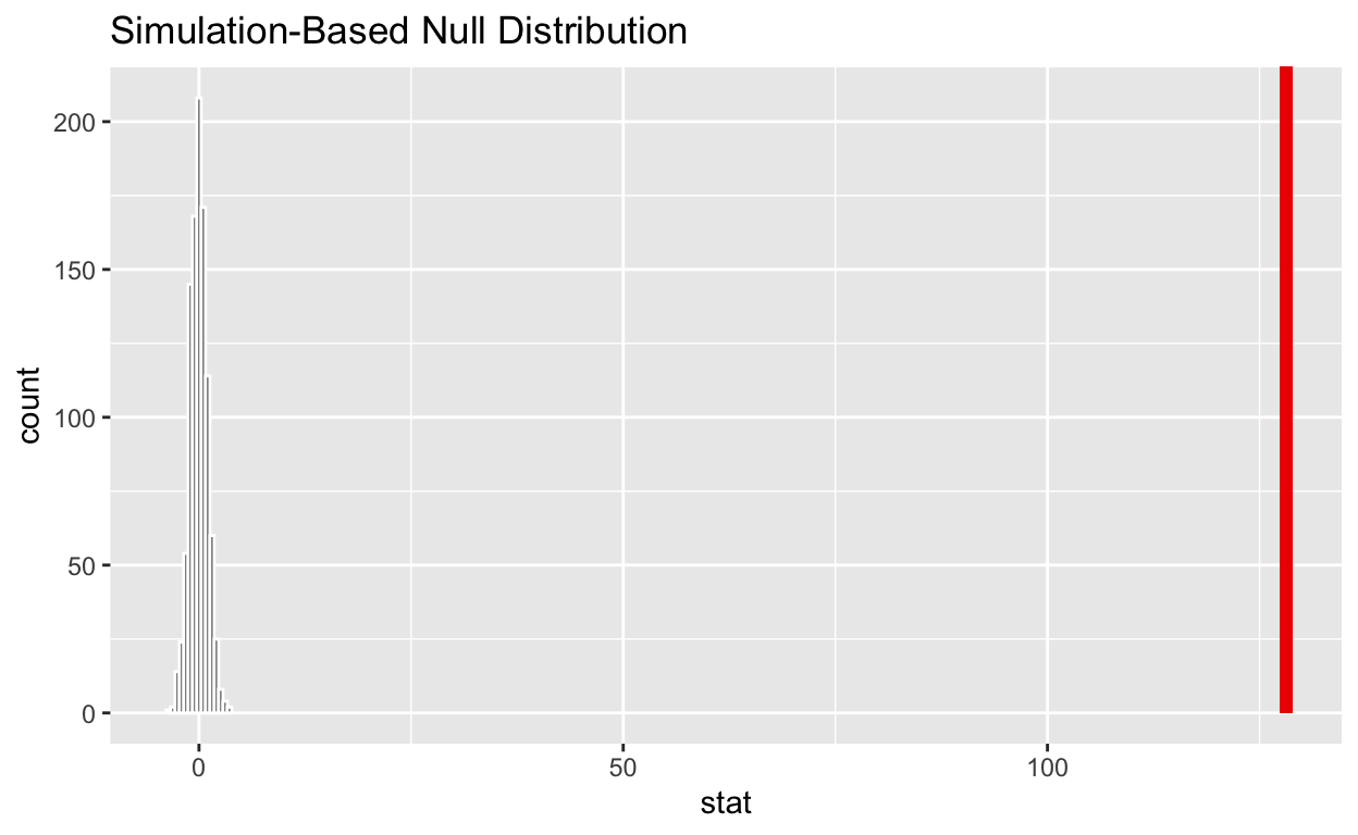
Save the previous plot to preview.png and add to the yaml chunk at the top

ggsave(filename = "preview.png", 
       path = here::here("_posts", "2022-04-11-hypothesis-testing"))

If the p-value < 0.05? yes

Does your analysis support the null hypothesis that the true means of the number of hours worked for those that were “fired”, “ok” and “promoted” were the same? no