Project Part II

Interactive and static data plots of source type CO2 emissions from 1920 to 2000.

1. Install packages we will use to read in and plot the data.

library(tidyverse)
library(echarts4r)

2. Read the data in from part I

source_type_co2 <- read_csv(here::here("source_type_co2.csv"))

Interactive Graph

• Start with the data
• Use pivot_longer to show columns as source types of CO2 within the world.
• group_by source so there will be an indication for each CO2 emission source type.
• Use mutate to change Year so it will be displayed as end of year instead of the beginning of the year.
• Use e_charts to create an e_charts object wtih Year on the x-axis.
• Use e_river to create “rivers” that contain the amount of CO2 emissions for each source type.
• Use e_tooltip to add a tooltip that will display based on the axis values
• Use e_title to add a title, subtitle, and link to subtitle
• Use e_theme to change the theme to

source_type_co2 %>% 
  pivot_longer(cols = 2:7, names_to ="source_type", values_to = "amount") %>% 
  group_by(source_type) %>%
  mutate(Year = paste(Year, "12", "31", sep = "-")) %>% 
  e_charts(x = Year) %>% 
  e_river(serie = amount, legend=FALSE) %>%
  e_tooltip(trigger = "axis") %>% 
  e_title(text = "Annual CO2 Emissions, by source type",
          subtext = "(in billions of tonnes). Source: Our World in Data",
          sublink = "https://ourworldindata.org/grapher/co2-by-source",
          left = "center") %>% 
  e_theme("roma")

Static Graph

• Start with the data
• Use ggplot to create a new ggplot object. Use aes to indicate that Year will be the x-axis; CO2 emissions will be the y-axis; Source type will be fill variable.
• geom_area will display Source Type
• scale_fill_discrete_divergingx is a function in the colorspace package, this will set the color package to roma and selects a max of 12 colors to indicate the different source types.
• theme_classic sets the theme
• theme(legend.position = "bottom") puts the legend at the bottom of the plot
• labs sets the y-axis label, fill = NULL indicates that the fill variable will not have the labelled source type.

source_type_co2 %>% 
  pivot_longer(cols = 2:7, names_to ="source_type", values_to = "amount") %>% 
  group_by(source_type) %>% 
  ggplot(aes(x = Year, y = amount, fill=source_type)) +
  geom_area() +
  theme_classic() +
  theme(legend.position = "bottom") +
  labs( y = "in billions of tonnes",
        fill = NULL)

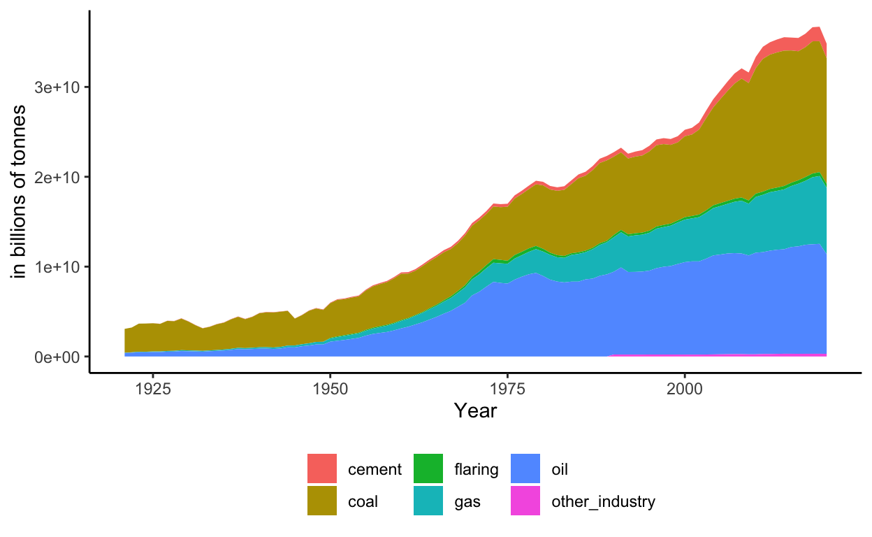
• These plots show a steady increase in the use of emissions since 1920. Emissions have continued to increase and expand different types of CO2 emissions resources.

ggsave(filename = here::here("_posts/2022-05-12-project-part-ii/preview.png"))